


Reset password
If you have forgotten your password, click on the "Forgot password" link in the login screen. Another dialog box will appear, in which you must enter your user name. Click on "Continue" and you will receive an email to the email address we have on file for you with a link that you can use to reset your password.


 | Gradually zooming in and out on the map. |
 | Search for your own location: The map section zooms in on the user's current location (if it can be determined via the IP address). |
 | The map window is set to the current default extent. This can be the whole of Germany or a regional section, depending on the extent of the integrated data. |
 | Selection of a background map from several different templates. |
The map section is always moved using the mouse (hold down the left mouse button). To do this, the mouse pointer must be in the map window.
 in the header at the top right.
Potential for locations (select locations)
The parameters for the function are specified in several steps.
Define location
The quickest way to define a location for which the potential is to be determined is to click on the map. First, the Add button (blue = active, gray = inactive) is activated to set a location on the map.

The mouse pointer changes to a cross symbol on the map. If you click on a location, its address is determined and listed in the dialog box.
- A total of up to 5 locations can be defined on the map. A message appears when the maximum number of locations has been reached.
- Locations can be removed from the list by clicking on the corresponding red cross. The red trash can button deletes all points set on the map.

Alternatively, you can also search by address. The text field at the top left of the map window can be used for this purpose. Even if parts of the address, such as the Postal code , are Postal code , the system will attempt to validate the address based on the information provided and generate a list of suggestions. The desired entry can then be selected from this list.

After selecting a hit or clicking on the magnifying glass, the map zooms in on the location. By clicking on the point, the address can be transferred directly to the list for potential determination via the pop-up window.

If the potential for multiple locations needs to be determined, a list of these addresses can be quickly and easily imported and displayed on the map using the Geocode Addresses function ( see chapter Geocoding Addresses).
The addresses can be added directly using the Transfer addresses button in the Determine potential function.
- If the list contains more than 5 addresses, the first 5 will be used as locations.
- If addresses have already been added, the list will only be supplemented up to a maximum of 5 locations.
Define catchment area
The next step is to define the catchment area for one or more locations.
The following modes are available:
- Radius: Straight-line distances are calculated. This method is quite fast, but depending on the geography (e.g., rivers without bridges, mountains), it can lead to unrealistic catchment areas.
- Routing: Distance zones are calculated on the road network (from the perspective of cars or pedestrians with different traffic rules such as one-way streets, turning regulations, etc.). This method takes longer, but results in more realistic catchment areas.
- Kilometers, meters, and minutes are available as units for distances per zone.

The distance values are then specified. When the value for a zone is entered, another field is added to the list. Up to 5 zones can be created with a total distance of up to 100 km or 60 minutes (for routing zones).
For the Routing Zone mode (calculation based on the road network) with the car as the mode of transport, a flexible speed profile can be specified. To do this, the average speeds for three road categories are set: city (within cities and towns), country roads (outside towns), and highways.

The standard profile with city (30 km/h), country road (60 km/h), and highway (110 km/h) is suitable for locations outside of metropolitan areas or outside of rush hour traffic times.
Within urban areas or during periods of heavy rush hour traffic, low values are recommended, e.g., city (15 km/h), country roads (30 km/h), and highways (70 km/h). These average values take into account all traffic light stops and temporary traffic jams. The values can be entered directly into the text fields for each category.
For pedestrians, a speed of 4 km/h is generally assumed, and for bicycles, a speed of 18 km/h is generally assumed.
Select variable
The next step is to select the variables (market data) on the basis of which the potential for each distance zone is to be determined.

Clicking on the Variables button opens the dialog box for selecting market data. Depending on your license, several associated geographic levels are available for selection.
There is a separate service for standard data (including population by age group, households, purchasing power, and company counters by industry). The data is available for three geographical levels: residential areas, postal codes, and municipalities.

In this example, the total number of inhabitants, the number of households (SUM column = totals), and the maximum purchasing power per inhabitant are selected as potentials.
To select a variable, click on the corresponding button in the column with the desired calculation method. The button for a variable remains blue as long as it is added to the selection.
- Sum: The sums of a numerical variable are calculated, e.g., for residents, households, or companies in a particular industry.
- Max: The maximum value of a numeric variable is determined.
- Min: The minimum value of a numeric variable is determined.
- Ø: The average value of a numerical variable is determined, e.g., for calculating the average purchasing power index.
- Anz: The number of objects within a zone is determined. This is available, for example, for counting Topshops (chain stores) that represent a special feature (not included in the standard).
Up to 10 variables can be added to the lower selection list. Data that has already been added can be removed again using the cross button. Another click on a blue button is also sufficient.
When the maximum number of variables has been reached, a message appears. No further variables can then be added.
The settings dialog box is closed by clicking the OK button. The number of selected variables is displayed next to the blue variables button.

Other calculation methods
Further specifications can be made for calculating the potentials.

- Consider table filters: In the data table for a geographic level, a filter can be set for each variable. This can be useful if, for example, only areas with high purchasing power are to be considered for the potential calculation, or only postal codes for a specific area (see chapter Table). These filters are taken into account by activating the option during the potential calculation. If no active filter is set in the data table for a geographic level, the option is deactivated.
The principle is explained in this graphic: without a filter, the number of inhabitants is determined for both intersecting areas – with a filter, however, only for the area that meets the criteria.

- Maximum or minimum potential: The maximum potential is used to determine the values for all area units intersected by the zones. The minimum potential is used to calculate the potentials according to the area share (percentage share) of an area within a zone.
The principle is explained in this diagram: With "Maximum," the values of the intersecting areas are allocated completely; with "Minimum," they are allocated only proportionally to the area share.

If no selection is made in the table filter, the set filters are not taken into account and the "maximum potential" is calculated.
- No overlap: This option is only available if the evaluation is carried out for two or more locations. Potential is thus clearly assigned to the nearest location (based on the center of the area) and is therefore not assigned twice or multiple times.

Identify potential
Each potential calculation created can be assigned an individual analysis name directly in the name input field (optional). If no analysis name is assigned, the default name is Potential Analysis Result.

The Start button executes the potential calculation for the created zones based on the selected variables (market data). Only then are the other options available.
- The distance zones created are displayed directly on the map after calculation. A new layer appears in the layer dialog box at the top left.

- The options menu (three-dot menu) on the right-hand side allows you to flexibly adjust settings such as transparency and zoom.
Results
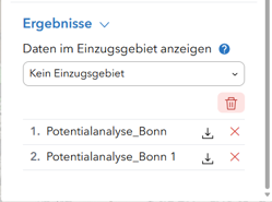
Under the "Results" tab, you can delete the zones you have created—for example, to rerun the calculation with different settings. The variables you previously selected will also be deleted.
About the download icon
 You have the option to export the calculated potential results as a report (in PDF format).
 You have the option to export the calculated potential results as a report (in PDF format).
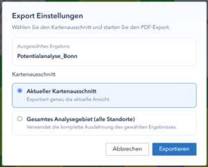
Create a report
- There are two options available for exporting:
- Current Map Section: Exports the current map view.
- Entire Analysis Area (All Locations): Exports the complete view of the created zones.
- The report consists of a cover page, an overview map, a legend, a table of potential values with zone statistics, and detailed maps of the watersheds.
For the newly created zone layer with the catchment area, the table with the determined potentials opens in the lower area. This table can also be sorted in ascending or descending order by column, or filters can be set for individual fields.

In this example, approximately 330,500 residents live within a one-minute zone of the location.
Map adjustment
By activating the Show data in catchment area option, only the units of the active layers that are intersected by the distance zone are displayed in the map window. This filters the data spatially.

Potential for an area ( draw area)
Potential data can also be determined based on any area that is interactively drawn on the map. The Draw Area option is available for this purpose.

- When a new polygon is drawn, the old area is automatically deleted. Only one area is valid at a time.

- Then, as for the Locations variant (select locations), the variables for determining potential are selected. Variables that have already been selected remain unchanged for this variant (see above).
- Similarly, the calculation methods are specified and the potential is determined (see above).
Geocoding addresses
The geocoding addresses function allows you to quickly and easily import address lists with customer or location addresses and display them on the map.
The function can be accessed directly via the button  in the header at the top right.
Through the geocoding process, addresses are first checked (validated) and then, if possible, enriched with location coordinates. As a result, a new geographic layer (point layer) appears on the map, in which the geocoded addresses and other variables from the input file (e.g., sales, etc.) are displayed in the attribute table. By clicking on the points on the map, the stored information can be retrieved.
Select file
The Select File button can be used to navigate to the file folder containing the address list that is to be geocoded. The input lists can be semicolon- or tab-separated text files ( CSV or TXT formats, best saved in UTF-8 due to possible umlauts) and contain up to 1,000 address entries including column headers.


Once the file has been selected, the file name is displayed below the button.
settings
The address list is imported using the Upload file button. The separator (semicolon or tab) for the address file is automatically recognized and set. If field names are in the first row (recommended), activate the option First row contains field names.

column assignment
The column assignment is generated automatically after import. For standard labels such as Zip code, city, and street, these fields are already preset.

If the house numbers are not in a separate column but together with the street names, the corresponding option can be activated. The assignment for the field with the house number is then deactivated.
The Preview tab can be used to check once again whether the information from the address list has been imported correctly.
result
The Start button starts the geocoding process. The geocoded addresses are then displayed on the map as point symbols.

In addition, the addresses are also displayed in table form below the map. The data can be sorted or filtered there using a column (see chapter Tables).
- Only one address table can be processed in the map project at a time. If a new address list is geocoded, the existing one in the map will be replaced.
- The layer can also be removed from the map using the Delete addresses button.
By clicking on a location icon on the map, the stored information can be interactively accessed in an info dialog.
Customize display
The display of geocoded addresses on the map can be changed using the Symbolization function (see Symbolization chapter). To do this, select the address layer with the geocoded addresses as a layer and color it accordingly using the field.
symbolization
Relevant key figures and variables can be presented in the form of thematic maps: What is the spatial distribution of purchasing power or a specific age group when viewed on a geographical level? The visualization (representation) can be optimally adapted to the question at hand. This allows you to define your own classes and create color scales.
This function can be accessed directly via the button symbolization  in the header at the top right.
Select level and field
First, select the geographic level and then the available field (variable) to be displayed on the map. There are 3 levels available by default:
Postal codes ( Zip code): approx. 8,200 Zip code.
Communities: approximately 11,200 communities.
Residential areas: 88 ,000 neighborhood areas

After setting the geographic level, select the field (variable). In this example, the residents are selected.
classes
The class boundaries can be adjusted in the Classes dialog box: For which values should the geographical units (e.g., residential areas or Zip code) be displayed in dark blue, and for which in light blue? This can be done directly by entering the values (minimum and maximum per class) in the fields and setting a design color.

In addition, clicking on one of the color boxes allows you to adjust the color display for a specific class. A color palette appears, from which you can select the desired color with a mouse click. The change in classification is immediately visible on the map after clicking the Apply button.

The width of the outlines for the geographic units on the map can also be adjusted. If a point layer (e.g., Topshops) is set as a geographic layer, the point size on the map can be adjusted.
If you disable the Fill option, only the outlines will be visible on the map. This can be helpful if you only want to display the boundaries of the area units (e.g., Zip code, residential districts, or municipalities) on the map.
Generate classes
On the Classes tab, you can also automatically create your own classes. To do this, set the number of classes, the classification method, and a color gradient (design color).
The number of classes indicates how many classes the data spectrum is divided into. The data can be divided into a maximum of 5 classes. In most cases, 3 to 5 classes are ideal.
The Design Color feature allows the data for the selected variable to be displayed on the map using a predefined color gradient.
In addition, two classification methods are available to automatically obtain a suggestion for class boundaries.

quantile
In this case, each class is assigned the same number of geographic units. It is suitable for data with a linear distribution where the values are distributed quite differently.
Equal interval
The class intervals remain constant: the difference between the highest and lowest values per class is the same for all classes. This is advantageous for data values such as percentages or temperature values.
Clicking Apply will immediately update the map display based on the specified settings.
Single color
The Single Color tab can be used to color the available layers and data sets in a uniform color scheme. To do this, a design color can be set using the color palette or by entering a HEX or RGB code.

Categories
The Categories tab allows you to color the available layers and data sets according to specific categories. This option is only available for fields containing text values. The Category option is disabled in columns with numeric values. Here, too, you can customize the color representation for a specific category by clicking on one of the color boxes. If the text column contains more than 50 categories, only the first 50 unique categories are displayed.

table
The tables with market data below the map window provide important tools for analyzing the geographic units in the map window.


- The tables for the layers active in the map are always displayed.
- For these, only the data records for the units currently visible in the map window are displayed.
basic functions
The table functions are described below.
| The Actions button on the far right can be used to access the functions Set filter, Statistics, and Zoom to current selection. |
| The highlighted color indicates which table is currently active. Only tables for currently visible layers are displayed. |
| This icon can be used to show or hide the columns/variables displayed in the table for a layer. |
| This button updates the table. |
| These buttons display the current selection in the table (and thus also on the map) and also cancel it. |
Sort and filter
Clicking on the column header of a variable allows you to sort the values in ascending or descending order. When sorting is enabled, a small triangle appears in the column header.
The Set Filter function can be used to limit the amount of data in the table. The filters set can be linked together using AND/OR relationships (AND/OR criteria).
Example: You are looking for postal codes with a high proportion of "best agers" and high purchasing power per inhabitant. The criteria are therefore:
Proportion of residents aged 50–64 > 20% AND purchasing power per resident > €25,000
- Clicking on the Actions button opens the filter dialog. Use Add to set the filter in the form of a clause or a set of clauses.

- Clause (simple filter): simplest form of a filter with a single condition
- Clause set (multiple filters): Combination of multiple filters linked by an AND-OR relationship
- For our example, select "Clause rate" as the filter option. The AND relationship is preset in the filter dialog box that opens. In the next step, define the corresponding variables and limit values. Select "Proportion of residents aged 50–64 (%)" as the column, "is greater than" as the condition, and "20" as the value. The filter for the "Purchasing power per resident" attribute is specified accordingly in the lower filter dialog box.

Select source type
This option allows you to select the source type for defining the filter. There are three options to choose from:

- User input: allows values to be entered directly for filtering
- Field: filters based on the values in a specific attribute column
- Unique: displays a list of unique values in a specific attribute column that can be used for filtering
The filter in the table is activated using the upper Activate button (blue = filter active, white = filter inactive).

The number of records in the table is reduced accordingly. Only those Zip code that are currently visible in the map section and meet both criteria are Zip code .
The filters you have set can be removed by clicking on the same button. The data records for all units displayed in the map section will be shown again.
statistics
In the attribute table, you can display the statistics for a column for a level. The function is called up via the Actions button and the Statistics selection. In the Statistics dialog box, you can select one of the available columns for each active table.

In addition to our example of zip codes with a high proportion of "best agers" and high purchasing power per capita, the total and minimum and maximum number of households (in North Rhine-Westphalia) in the selected Zip code can also be Zip code . Other relevant statistical parameters would be the mean and standard deviation.